Horizontal diffusion of tracers

Lateral mixing due to mesoscale eddies is believed to occur according to this figure:

Horizontal surface boundary layer fluxes and interior epineutral fluxes.

We start by describing an implementation of the mixing in the interior and then introduce a surface mixed layer implementation. A bottom mixed layer implementation is planned for the future.

Epineutral Diffusion

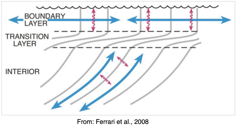
For the interior of the ocean, we would like to have horizontal diffusion with the following properties:

Suitable for general coordinate models
Preserves extrema
Has no need for regularization or tapering (such as needed by rotated mixing tensors)

The algorithm used in MOM6 is described by [31] and will be introduced here. The aim is to allow lateral mixing of tracers within isopycnal layers. It is appropriate for the adiabatic interior of the ocean while a lateral mixing scheme for the surface boundary layer is described below.

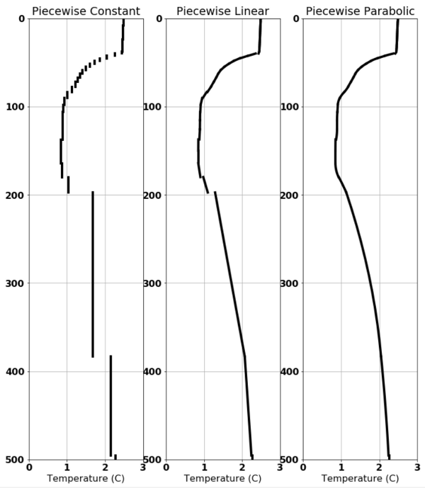
Before presenting this scheme, a quick review of polynomial reconstructions is in order. Some choices for the vertical representation of a finite volume quantity are shown here:

Polynomial reconstructions, starting with piecewise constant on the left, piecewise linear in the middle and piecewise parabolic on the right.

Some desired quantities for the polynomial reconstructions to be used are:

Tracer concentrations represent the cell-averages in vertical discretization.
Must be monotonic and introduce no new extrema.
Discontinuous reconstructions are desirable to limit intracell slopes.

The algorithm has three phases: initialization, sorting, and flux calculation.

Initialization

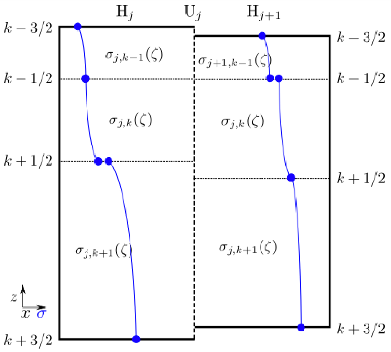
We begin by generating polynomial reconstructions of the vertical tracer quantities such as shown by the blue lines here:

Polynomial reconstructions of two adjacent water columns.

Because we are looking to mix along epineutral surfaces, we will need to find surfaces of uniform density by using the temperature, salinity, and their effect on the density, $\alpha$ and $\beta$. The next step is to find the values of $\alpha$ and $\beta$ at the interfaces.

Also during the initialization, the unstable parts of the water column are set aside to be skipped by this algorithm.

Sorting

The epineutral surfaces have constant density, where we use this equation:

\[ \Delta \rho = \rho_1 - \rho_2 = \frac{\alpha_1 + \alpha_2}{2} (T_1 - T_2) + \frac{\beta_1 + \beta_2}{2} (S_1 - S_2) \]

When calculating $\alpha$ and $\beta$, there's more than one way to do it. Using a midpoint pressure gives neutral density while using a reference pressure gives isopycnal values.

Given two adjacent water columns, we are going to be looking to match densities. The match does not need to be at the same level or even near each other in depth. Starting from the top two interfaces, search the column with the lighter surface water (second column) downward to find which layer contains water matching that of the first column at the surface:

Searching the column with the lighter surface for the water matching the other column's surface water.

If the surface density matches that of an interface, point to the interface. Otherwise, solve for the matching density along the polynomial reconstruction for that layer. There are again some choices:

Use Newton's method to find the root with higher order polynomials.
Assume $\alpha$ and $\beta$ vary linearly from top to bottom (cubic if $T$ and $S$ are parabolic).
Equation of state is linear from top to bottom interface (parabolic of $T$ and $S$ are parabolic).
$\Delta \rho$ is linear in the vertical.

Once the location of the first column's surface density is found in the second column, one goes to the next interface below to find the bottom density of the water to be mixed. Then find that density within the first column. Iterate downward until no more matches are found. These pairs of surfaces make up what is known as a sublayer along which the diffusion can take place.

Flux Calculation

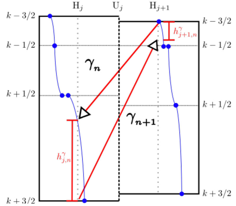
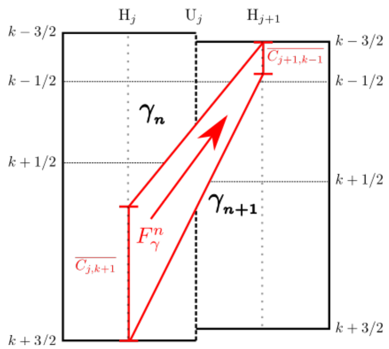
For each sublayer, the fluxes are based on the mean tracer quantities within that sublayer in each column. For a tracer $C$, compute the vertical average of that tracer within the sublayer to form $\overline{C}$. The flux can then be computed based on:

\[ F = K h_{\mbox{eff}} \frac{\overline{C_{j,k+1}} - \overline{C_{j+1,k-1}} }{\Delta x} \Delta t \]

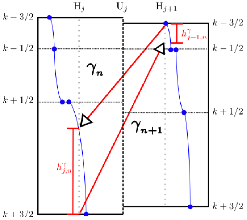
where the effective thickness of the sublayer is:

\[ h_{\mbox{eff}} = \frac{2 h_{j,n}^\gamma h_{j,n+1}^\gamma}{h_{j,n}^\gamma + h_{j,n+1}^\gamma} \]

and as shown in this figure:

Diagram of sublayer thickness for the sublayer bounded by surfaces $$ and ${n+1}$.

Flux of tracer $C$ along the sublayer.

When updating the tracer state, one needs to accumulate all the fluxes through each face as shown here:

Accumulate all the fluxes across a face from all the layers in the next column contributing to it.

Surface Diffusion

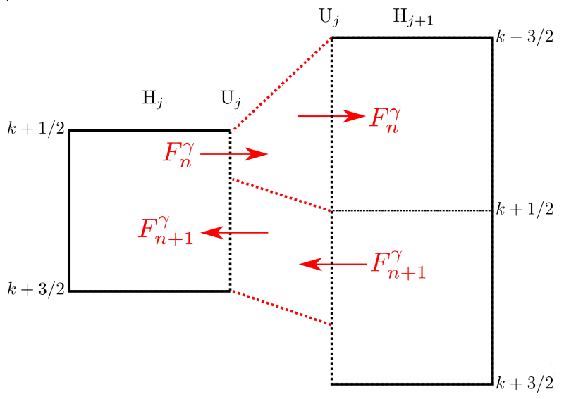
As shown in figure eddy_flux of the eddy fluxes, the diffusion in the surface boundary layer is assumed to be purely horizontal. A bulk scheme was explored but found wanting, so a layer-by-layer approach has been implemented instead. It is this layer-by-layer code which is described here.

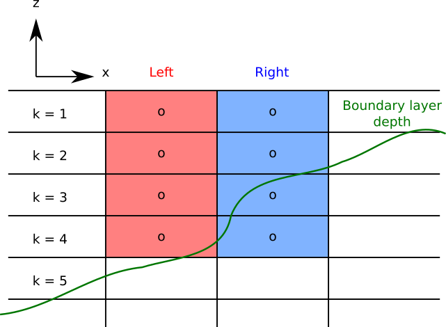
For each water column, the boundary layer thickness is determined first. This can be either via the CVMIX boundary layer thickness or through some other means. Next, determine how many of the model layers are within this boundary layer thickness. It is common for neighboring cells to have differing numbers of layers within the surface boundary layer, such as shown here:

Two cells within the surface mixed layer, red on the left, blue on the right. The mixed layer depth is shown in green.

In this case, the cell on the left has four layers within the boundary layer while the cell on the right has just two. The layer-by-layer scheme computes fluxes for the first two layers, then has linearly reduced fluxes for the next two layers below as shown here:

Two cells within the surface mixed layer with down-gradient fluxes as shown by the black arrows.

In all cases, the tracer flux is always down-gradient.

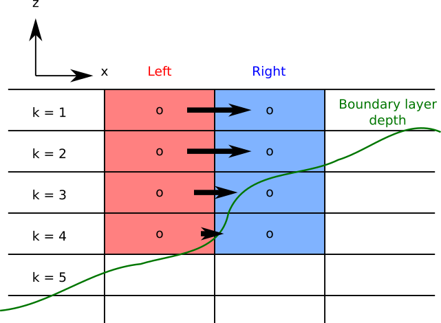
\[ F(k) = K h_{\mbox{eff}(k)} \left[ \phi_L(k) - \phi_R(k)\right] \]

where the effective thickness of the layer $k$ is:

\[ h_{\mbox{eff}(k)} = \frac{2 h_{L}(k) h_{R}(k)} {h_{L}(k) + h_{R}(k)} \]