|
MOM6
|


|
|
MOM6
|
|
Time-averaged accelerations
The barotropic equations are timestepped with a timestep to resolve the surface gravity waves. With care, the baroclinic timestep only need resolve the inertial oscillations. The barotropic accelerations are averaged over the many barotropic timesteps taken between baroclinic steps. At time \(n\), the baroclinic accelerations are computed. The vertical average of that acceleration is subtracted off and replaced by the time-averaged acceleration from the group of barotropic timesteps:
\[ \Delta t \frac{\partial \vec{u}}{\partial t} = \Delta t \left( \frac{\partial \vec{u}}{\partial t} - \frac{\partial \vec{u}_{BT}}{\partial t} \right)^n + \Delta t \overline{\frac{\partial \vec{u}_{BT}}{\partial t}}^{\Delta t} \]
Similarly, the velocities used in the tracer equation are a careful blend of the barotropic and baroclinic solutions:
\[ \Delta t \frac{\partial \theta}{\partial t} + \Delta t \left( \tilde{\vec{u}} \cdot \nabla \theta + \widetilde{w} \frac{\partial \theta}{\partial z} \right) \]
with
\[ \tilde{\vec{u}} = \vec{u}_{BC} + \overline{\vec{u}_{BT}}^{\Delta t} \]
\[ \frac{\partial \widetilde{w}}{\partial z} = - \nabla \cdot \tilde{\vec{u}} \]
The vertically discrete, temporally continuous layer continuity equations are:
\[ \frac{\partial h_k}{\partial t} = - \nabla \cdot (\vec{u} h_k) = - \nabla \cdot \mathbf{F} (u_k, h_k) \]
The relationship between the free surface height and the layer thicknesses \(h_k\) is:
\[ \eta = \sum_{k=1}^N h_k - D \]
We get an evolution equation for the free surface height:
\[ \frac{\partial \eta}{\partial t} = \sum_{k=1}^N \frac{\partial h_k}{\partial t} = - \nabla \cdot \sum_{k=1}^N \mathbf{F} (u_k, h_k) \]
If the algorithms for the fluxes in the continuity equations are linear in the velocity, the free surface height can be rewritten as:
\[ \frac{\partial \eta}{\partial t} \&= - \nabla \cdot \sum_{k=1}^N \mathbf{F} (u_k, h_k) = - \nabla \cdot \sum_{k=1}^N (\vec{u}_k h_k) \\ \&= - \nabla \cdot \left[ \sum_{k=1}^N h_k \frac{\sum_{k=1}^N (\vec{u}_k h_k)} {\sum_{k=1}^M k_k} \right] \equiv - \nabla \cdot H \mathbf{U} \]
where
\[ \mathbf{U} \equiv \frac{\sum_{k=1}^N (\vec{u}_k h_k)} {\sum_{k=1}^M k_k} \]
\[ H \equiv \sum_{k=1}^N h_k \]
However, ALE models like MOM6 require positive-definite, nonlinear continuity solvers (MOM6 uses PPM Advection Scheme). We need a different way to reconcile this estimate of free surface height with the one coming from the barotropic equations. After rejecting several other options, MOM6 is now using the scheme from [17]. The barotropic update of \(\eta\) is given by:
\[ \frac{\eta^{n+1} - \eta^n}{\Delta t} + \nabla \cdot \left( \overline{UH} \right) = 0 \]
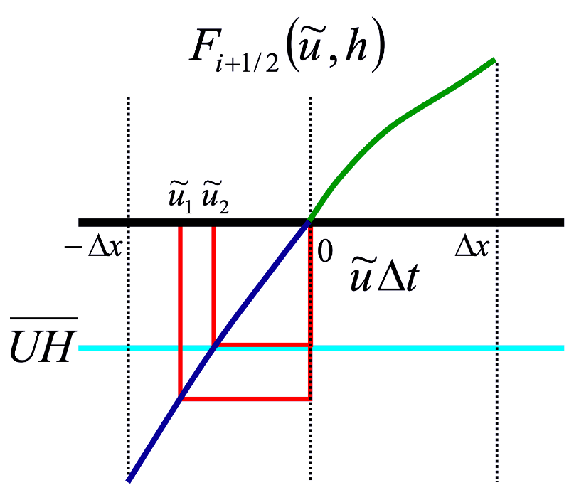
Determine the \(\Delta U\) such that:
\[ \sum_{k=1}^N \mathbf{F} (\tilde{u}_k, h_k) = \left( \overline{UH} \right) \]
where
\[ \tilde{u}_k = u_k + \Delta U \]
The layer timestep equation becomes:
\[ h_k^{n+1} = h_k^n - \Delta t \nabla \cdot \mathbf{F} (\tilde{u}_k, h_k) \]
This scheme has these properties:
The solution is unique provided that:
\[ \frac{\partial}{\partial \tilde{u}_k} \mathbf{F}(\tilde{u}_k, h_k) > 0 \]
This is a reasonable requirement for any discretization of the continuity equation. In the continuous limit, \(\mathbf{F} (u,h) = uh\), so one interpretation is:
\[ \frac{\partial}{\partial \tilde{u}_k} \mathbf{F}(\tilde{u}_k, h_k) = h_{k,\mbox{Marginal}} \]
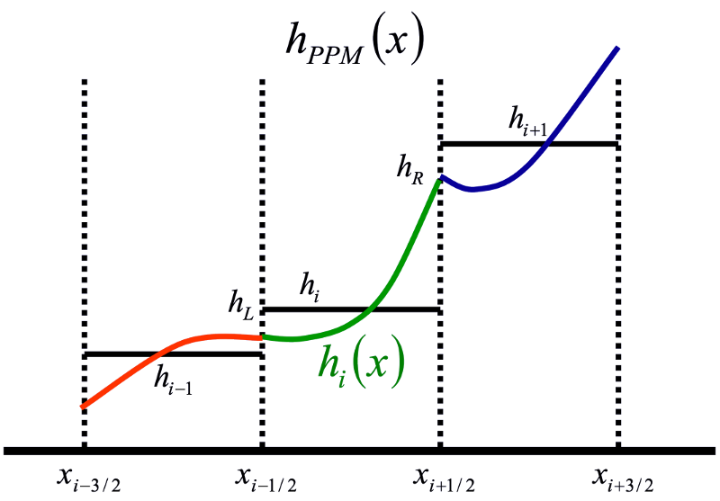
With the PPM continuity scheme:
\[ F_{i+1/2} = \frac{1}{\Delta t} \int_{x_{i+1/2} - u \Delta t}^{x_{i+1/2}} h_i^n (x) dx \]
leads to:
\[ \frac{\partial F_{i+1/2}}{\partial u_{i+1/2}} = h_i^n ( x_{i+1/2} - u_{i+1/2} \Delta t ) \equiv h_{k, \mbox{Marginal}} \]
\(h_i(x) > 0\) is already required for positive definiteness.
Newton's method iterations quickly give \(\Delta U\):
\[ \Delta U^{m+1} = \Delta U^m + \frac{\left( \overline{UH} \right) - \sum_{k=1}^N F(u_k + \Delta U^m, h_k)}{\sum_{k=1}^N h_{k,\mbox{Marginal}}} \]
The piecewise parabolic method continuity solver uses two steps:
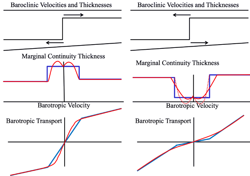
Barotropic accelerations do not lead to barotropic flows after a timestep when vertical viscosity is taken into account.
\[ u_k^{n+1} = u_k^n + \Delta t A_k + \Delta t \frac{\tau_{k-1/2} - \tau_{k+1/2}}{h_k} \]
\[ \tau_{1/2} = \tau_{Wind} \]
\[ \tau_{k+1/2} = \nu_{k+1/2} \frac{u_k^{n+1} - u_{k+1}^{n+1}}{h_{k+1/2}} \]
\[ \tau_{N+1/2} = \nu_{N+1/2} \frac{2 u_N^{n+1}}{h_{N+1/2}} \]
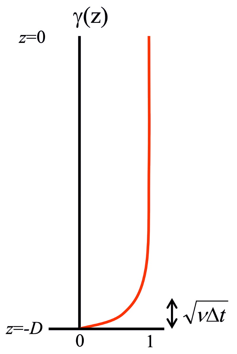
\[ \gamma_k \equiv \frac{1}{\Delta t} \frac{\partial u_k^{n+1}} {\overline{\partial A}} \]
A tridiagonal equation for \(\gamma_k\) results, going from 0 for thin layers near the bottom to 1 far above the bottom.
\[ \gamma_1 = 1 + \frac{1}{h_1} \left[ - \frac{\nu_{3/2} \Delta t}{h_{3/2}} (\gamma_1 - \gamma_2) \right] \]
\[ \gamma_k = 1 + \frac{1}{h_k} \left[ \frac{\nu_{k-1/2} \Delta t}{h_{k-1/2}} (\gamma_{k-1} - \gamma_k) - \frac{\nu_{k+1/2} \Delta t}{h_{k+1/2}} (\gamma_k - \gamma_{k+1}) \right] \]
\[ \gamma_N = 1 + \frac{1}{h_N} \left[ \frac{\nu_{N-1/2} \Delta t}{h_{N-1/2}} (\gamma_{N-1} - \gamma_N) - \frac{2\nu_{N+1/2} \Delta t}{h_{N+1/2}} \gamma_N \right] \]
In the continuous limit:
\[ \gamma(z) = 1 + \Delta t \frac{d}{dz} \left( \nu \frac{d \gamma}{dz} \right) \]
with boundary conditions:
\[ \frac{d \gamma}{dz} (0) = 0 \]
\[ \gamma(-D) = 0 \]
For deep water and contant \(\nu\), we get:
\[ \gamma (z) = 1 - \exp \left( - \sqrt{\nu \Delta t} (z + D) \right) \]
From above, the barotropic equation is:
\[ \frac{\eta^{n+1} - \eta^n}{\Delta t} + \nabla \cdot \left( \overline{UH} \right) = 0 \]
We need to determine the \(\Delta \overline{A}\) such that:
\[ \sum_{k=1}^N \mathbf{F} (\tilde{u}_k, h_k) = \left( \overline{UH} \right) \]
where
\[ \tilde{u}_k = u_k + \gamma_k \Delta \overline{A} \Delta t \]
\[ \frac{\partial \eta}{\partial t} = \nabla \cdot \overline{U} + M \]
\[ \overline{U} (\overline{u}) = \frac{1}{\Delta t} \int_0^{\overline{u} \Delta t} H(x) dx \]
\[ \overline{u}^n = \overline{U}^{-1} \left( \sum_{k=1}^N U_k^n \right) \]
\[ u_k^{n+1} = \tilde{u}_k^{n+1} + \Delta \overline{u} \]
We need to find \(\Delta \overline{u}\) such that:
\[ \sum_{k=1}^N U_k \left( \tilde{u}_k^{n+1} + \Delta \overline{u} \right) = \overline{U}^{n+1} \]
\[ \frac{\partial \overline{u}}{\partial t} \&= - f \hat{k} \times (\overline{u} - \overline{u}_{Cor}) - \nabla \overline{g} (\eta - \eta_{PF}) - \\ \& \frac{c_D \left( ||u_{Bot}|| + ||u_{Shelf}|| \right)}{\sum_{k=1}^N h_k} (\overline{u} - \overline{u}_{Drag}) + \frac{\sum_{k=1}^N h_k \frac{\partial u_k}{\partial t}} {\sum_{k=1}^N h_k} \]
 1.8.13